

Tutorial 2 - POA Irradiance & Module Temperature#
This notebook shows how to use pvlib to transform the three irradiance components (GHI, DHI, and DNI) into POA irradiance, the main driver of a PV system. Then this POA and weather data will be used to calculate Module Temperature

PV Concepts#
Plane of Array Irradiance
Angle of Incidence
Time delta for solar position
GHI vs POA for fixed tilt system and tracked systems
Module temperature and it’s dependence on POA and wind
Python Concepts#
pandas Timedelta
making a new dataframe from existing columns
resampling
bar ploting
What is transposition?#
The amount of sunlight collected by a PV panel depends on how well the panel orientation matches incoming sunlight. For example, a rooftop array facing West will produce hardly any energy in the morning when the sun is in the East because the panel can only “see” the dim part of the sky away from the sun.

As the sun comes into view and moves towards the center of the panel’s field of view, the panel will collect more and more irradiance. This concept is what defines plane-of-array irradiance – the amount of sunlight available to be collected at a given panel orientation. Like the three “basic” irradiance components, POA irradiance is measured in watts per square meter.
Each irradiance component is considered separately when modeling POA irradiance. For example, calculating the component of direct irradiance (DNI) that is incident on a panel is solved with straightforward geometry based on the angle of incidence. Finding the POA component of diffuse irradiance (DHI) is more complex and can vary based on atmospheric conditions. Many models, ranging from simple models with lots of assumptions to strongly empirical models, have been published to transpose DHI into the diffuse POA component. A third component of POA irradiance is light that reflects off the ground before being collected by the PV panel. Functions to calculate each of these components are provided by pvlib.

How is array orientation defined?#
Two parameters define the panel orientation, one that measures the cardinal direction (North, East, South, West), and one that measures how high in the sky the panel faces:
tilt; measured in degrees from horizontal. A flat panel is at tilt=0 and a panel standing on its edge has tilt=90.
azimuth; measured in degrees from North. The direction along the horizon the panel is facing. N=0, E=90, S=180, W=270.
A fixed array has fixed tilt and azimuth, but a tracker array constantly changes its orientation to best match the sun’s position. So depending on the system configuration, tilt and azimuth may or may not be time series values.
Now to Code:#
0. Step 0 If running on Google Collab:#
If running on google colab, uncomment the next cell and execute this cell to install the dependencies and prevent “ModuleNotFoundError” in later cells:
# !pip install -r https://raw.githubusercontent.com/PV-Tutorials/2024_PVSC/requirements.txt
1. Import your libraries#
import pvlib
import pandas as pd  # for data wrangling
import matplotlib.pyplot as plt  # for visualization
import pathlib  # for finding the example dataset

print(pvlib.__version__)
---------------------------------------------------------------------------
ModuleNotFoundError                       Traceback (most recent call last)
Cell In[2], line 1
----> 1 import pvlib
      2 import pandas as pd  # for data wrangling
      3 import matplotlib.pyplot as plt  # for visualization

ModuleNotFoundError: No module named 'pvlib'
2. Download the Weather Data you will use#
We are making you code. Go to tutorial 1, and copy the lines you need to download the weather data:
# Hint 1: You will need the API
# Hint 2: You will need the get_psm3 function call
If you have succeeded in copy-pasting the above, congratulations, you ARE Coding!
3. Calculate Sun Position#
# make a Location object corresponding to this TMY
location = pvlib.location.Location(latitude=metadata['latitude'],
                                   longitude=metadata['longitude'])
0.9.4.dev19+ge4356f9
print("We are looking at data from ", metadata['Name'], ",", metadata['State'])
We are looking at data from "GREENSBORO PIEDMONT TRIAD INT" , NC
solar_position = location.get_solarposition(times)
PSA: Because part of the transposition process requires knowing where the sun is in the sky, let’s use pvlib to calculate solar position. There is a gotcha here! Depending on the source of your weather data and how it was averaged, you might need to calculate solar position at the specific position of the timestamp, or at the middle of the previous or current hour.#
NSRDB provides irradiance data at the middle of the hour already, so sun position should be calculated at that exact time. TMY3, now deprecated, used to average data ‘right labeled’, so the sun should be calculated 30 minutes before. What does PVGis data does?
But that is not the only factor to consider. Softwares have certain expectations on the input data unless you specify otherwise. SAM expects data to be left labeled, unless you provide minute data in which case it models at the specific timestamp given. PVSyst expects data left labeled, unless you use their data loading setup and specify this is not the case. PVlib will calculate sun position at the timestamp given.
This issue trips most modelers, as shown by the many international round-robins, and can cause discrepancies on sun position, tracker position, and energy yield.
Pvlib calculates solar position for the exact timestamps you specify. The following code example shows how to adjust the times by half an hour, in case it is needed:
times = df_tmy.index - pd.Timedelta('30min')
solar_position = location.get_solarposition(times)
solar_position.index += pd.Timedelta('30min') # but remember to shift the index back to line up with the TMY data:
The two values needed here are the solar zenith (how close the sun is to overhead) and azimuth (what direction along the horizon the sun is, like panel azimuth). The difference between apparent_zenith and zenith is that apparent_zenith includes the effect of atmospheric refraction.
Now that we have a time series of solar position that matches our irradiance data, let’s run a transposition model using the convenient wrapper function pvlib.irradiance.get_total_irradiance. The more complex transposition models like Perez and Hay Davies require additional weather inputs, so for simplicity we’ll just use the basic isotropic model here, which is the default if nothing is passed for model keyword argument. As an example, we’ll model a fixed array tilted south at 20 degrees.
4. Calculate fixed Tilt POA#
df_poa = pvlib.irradiance.get_total_irradiance(
    surface_tilt=20,  # tilted 20 degrees from horizontal
    surface_azimuth=180,  # facing South
    dni=df_tmy['DNI'],
    ghi=df_tmy['GHI'],
    dhi=df_tmy['DHI'],
    solar_zenith=solar_position['apparent_zenith'],
    solar_azimuth=solar_position['azimuth'],
    model='isotropic')
get_total_irradiance returns a DataFrame containing each of the POA components mentioned earlier (direct, diffuse, and ground), along with the total in-plane irradiance.
df_poa.keys()
Index(['poa_global', 'poa_direct', 'poa_diffuse', 'poa_sky_diffuse',
       'poa_ground_diffuse'],
      dtype='object')
What angle should you tilt your modules at?#
PVEducation Solar Radiation on a Tilted Surface
Model poa again, but now at a surface_tilt of 30 degrees
df_poa2 = pvlib.irradiance.get_total_irradiance( ....
  Cell In[1], line 1
    df_poa2 =
             ^
SyntaxError: invalid syntax
df = pd.DataFrame({
    'poa_20': df_poa['poa_global'],
    'poa_30': df_poa2['poa_global'],
})
df_monthly = df.resample('M').sum()
df_monthly.plot.bar()
plt.ylabel('Monthly Insolation [W h/m$^2$]');
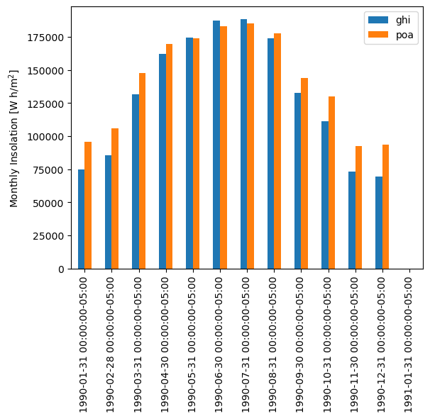
This plot shows that, compared with a flat array, a tilted array receives significantly more insolation in the winter. However, it comes at the cost of slightly less insolation in the summer. The difference is all about solar position – tilting up from horizontal gives a better match to solar position in winter, when the sun is low in the sky. However it gives a slightly worse match in summer when the sun is very high in the sky.
As an example, here’s a sunny day in winter vs a sunny day in summer. Note that the daily profile doesn’t just change its height, it also changes its width (summer POA is “skinnier” than GHI).
df.loc['1990-01-15'].plot()
plt.ylabel('Irradiance [W/m$^2$]');
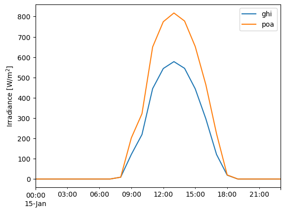
The difference between GHI and POA is of course dependent on the tilt defining POA, but because it also depends on solar position, it varies from location to location. Luckily, tools like pvlib make it easy to model!
4. Modeling POA for a tracking system#
The previous section calculated the transposition assuming a fixed array tilt and azimuth. Now we’ll do the same for a tracking array that follows the sun across the sky. The most common type of tracking array is what’s called a single-axis tracker (SAT) that rotates from East to West to follow the sun. We can calculate the time-dependent orientation of a SAT array with pvlib:
tracker_data = pvlib.tracking.singleaxis(
    solar_position['apparent_zenith'],
    solar_position['azimuth'],
    axis_azimuth=180,  # axis is aligned N-S
    )  # leave the rest of the singleaxis parameters like backtrack and gcr at their defaults
tilt = tracker_data['surface_tilt'].fillna(0)
azimuth = tracker_data['surface_azimuth'].fillna(0)

# plot a day to illustrate:
tracker_data['tracker_theta'].fillna(0).head(24).plot()
plt.ylabel('Tracker Rotation [degrees]');
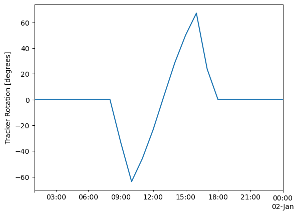
This plot shows a single day of tracker operation. The y-axis shows the tracker rotation from horizontal, so 0 degrees means the panels are flat. In the morning, the trackers rotate to negative angles to face East towards the morning sun; in the afternoon they rotate to positive angles to face West towards the evening sun. In the middle of the day, the trackers are flat because the sun is more or less overhead.
Now we can model the irradiance collected by a tracking array – we follow the same procedure as before, but using the timeseries tilt and azimuth this time:
df_poa_tracker = pvlib.irradiance.get_total_irradiance(
    surface_tilt=tilt,  # time series for tracking array
    surface_azimuth=azimuth,  # time series for tracking array
    dni=df_tmy['DNI'],
    ghi=df_tmy['GHI'],
    dhi=df_tmy['DHI'],
    solar_zenith=solar_position['apparent_zenith'],
    solar_azimuth=solar_position['azimuth'])
tracker_poa = df_poa_tracker['poa_global']
Let’s compare GHI and POA:
df.loc['1990-01-15', 'ghi'].plot()
tracker_poa.loc['1990-01-15'].plot()
plt.legend()
plt.ylabel('Irradiance [W/m$^2$]');
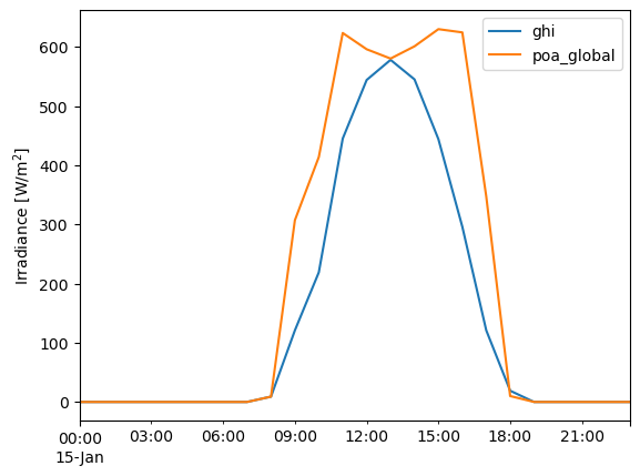
Notice how different the daily profile is for the tracker array! This is because the array can tilt steeply East and West to face towards the sun in early morning and late afternoon, meaning the edges of day get much higher irradiance than for a south-facing array.
Note also that in the middle of the day, GHI and POA just touch each other – this is because at solar noon, the array lies flat, and so POA is momentarily identical to GHI.
Note that the POA calculations discussed above do not address the partial blocking of diffuse light in arrays with multiple tilted rows of PV modules, so the results will be slightly (typically 1-3%) optimistic relative to real conditions or to commercial modeling software. Such corrections are likely to be added to pvlib in the future for specific generic geometries like fixed racks.
V. Model Temperature#
Now that we have the necessary weather inputs, all that is left are the thermal parameters. These characterize the thermal properties of the module as well as the module’s mounting configuration. Parameter values covering the common system designs are provided with pvlib:
all_parameters = pvlib.temperature.TEMPERATURE_MODEL_PARAMETERS['sapm']
list(all_parameters.keys())
open_rack_glass_polymer is appropriate for many large-scale systems (polymer backsheet; open racking), so we will use it here:
parameters = all_parameters['open_rack_glass_polymer']
# note the "splat" operator "**" which expands the dictionary "parameters"
# into a comma separated list of keyword arguments
cell_temperature = pvlib.temperature.sapm_cell(
    tracker_poa, df_tmy['DryBulb'], df_tmy['Wspd'], **parameters)
Now let’s compare ambient temperature with cell temperature. Notice how our modeled cell temperature rises significantly above ambient temperature during the day, especially on sunny days:
df_tmy['DryBulb'].head(24*7).plot()
cell_temperature.head(24*7).plot()
plt.grid()
plt.legend(['Dry Bulb', 'Cell Temperature'])
# note Python 3 can use unicode characters like the degrees symbol
plt.ylabel('Temperature [°C]');
Wind speed also has an effect, but it’s harder to see in a time series plot like this. To make it clearer, let’s make a scatter plot:
temperature_difference = cell_temperature - df_tmy['DryBulb']
plt.scatter(tracker_poa, temperature_difference, c=df_tmy['Wspd'])
plt.colorbar()
# note you can use LaTeX math in matplotlib labels
# compare \degree" with the unicode symbol above
plt.ylabel('Temperature rise above ambient [$\degree C$]')
plt.xlabel('POA Irradiance [$W/m^2$]');
plt.title('Cell temperature rise, colored by wind speed');
The main trend is a bigger temperature difference as incident irradiance increases. However, this plot shows that higher wind speed reduces the effect – faster wind means more convective cooling, so a lower cell temperature than it would be in calm air.
Note: the gap at the upper edge of the trend is an artifact of the low resolution of wind speed values in this TMY dataset; there are no values between 0 and 0.3 m/s.

This work is licensed under a Creative Commons Attribution 4.0 International License.