1 - Beginner - Plot Spectra and Albedos from SMARTS

1 - Beginner - Plot Spectra and Albedos from SMARTS#

Generate & Plot Spectra and Albedos from SMARTS#

* 1. DNI and DHI for a particular time and location#

* 2. Ground Albedo for various materials at AM 1.5#

* 3. Ground Albedo for complete AOD and PWD Weather Data#

try:
  import google.colab
  IN_COLAB = True
except:
  IN_COLAB = False

if IN_COLAB:
    !pip install -r https://raw.githubusercontent.com/PV-Tutorials/2024_pySMARTS_UNSA/main/requirements.txt

import numpy as np
import pandas as pd
import matplotlib.pyplot as plt
from matplotlib import style
import pvlib
import datetime
import pprint
import os
import pySMARTS

---------------------------------------------------------------------------
ModuleNotFoundError                       Traceback (most recent call last)
Cell In[2], line 5
      3 import matplotlib.pyplot as plt
      4 from matplotlib import style
----> 5 import pvlib
      6 import datetime
      7 import pprint

ModuleNotFoundError: No module named 'pvlib'

# Información para ayudar con errores
import sys, platform
print("Working on a ", platform.system(), platform.release())
print("Python version ", sys.version)
print("Pandas version ", pd.__version__)
print("pySMARTS version ", pySMARTS.__version__)

Working on a  Windows 10
Python version  3.12.4 | packaged by Anaconda, Inc. | (main, Jun 18 2024, 15:03:56) [MSC v.1929 64 bit (AMD64)]
Pandas version  2.2.2
pySMARTS version  0.0.1a1.dev14+g1573ee8.d20241128

if IN_COLAB:
    SMARTSPATH = r'SMARTS_295_PC'
else:
    SMARTSPATH = r'C:\SMARTS_295_PC'

SMARTSPATH = r'C:\Users\sayala\Documents\GitHub\py-SMARTS\SMARTS'

1. Obtener DNI y DHI para un lugar y tiempo en específico#

IOUT = '2 3' # DNI and DHI

YEAR = '2021'
MONTH = '06'
DAY = '21'
HOUR = '12'
LATIT = '33'
LONGIT = '-110'
ALTIT = '0.9' # km encima del nivel del mar
ZONE = '-7' # Timezone

pySMARTS.SMARTSTimeLocation(IOUT,YEAR,MONTH,DAY,HOUR, LATIT, LONGIT, ALTIT, ZONE, SMARTSPATH=SMARTSPATH)

	Wvlgth	Direct_normal_irradiance	Difuse_horizn_irradiance
0	280.0	2.698000e-18	4.531000e-19
1	280.5	3.907000e-17	6.666000e-18
2	281.0	1.579000e-16	2.638000e-17
3	281.5	2.278000e-15	3.841000e-16
4	282.0	1.135000e-14	1.893000e-15
...	...	...	...
1997	3980.0	7.564000e-03	1.467000e-07
1998	3985.0	7.558000e-03	1.467000e-07
1999	3990.0	7.478000e-03	1.441000e-07
2000	3995.0	7.356000e-03	1.403000e-07
2001	4000.0	7.089000e-03	1.338000e-07

2002 rows × 3 columns

Exercicio: Cambia ahora para tu latitud y longitud:

YEAR = '2021'
MONTH = '06'
DAY = '21'
HOUR = '12'
LATIT = 
LONGIT = 
ALTIT = '0.9' # km above sea level
ZONE = 

mi_espectra = pySMARTS.SMARTSTimeLocation(IOUT,YEAR,MONTH,DAY,HOUR, LATIT, LONGIT, ALTIT, ZONE, SMARTSPATH=SMARTSPATH)

Los resultados no se imprimieron en la pantalla porque se grabaron en la variable mi_espectra.

Pero ahora podemos usar esa variabla para hacer gráficos. Primero, va a ser útil saber el nombre de las columnas que obtuve

mi_espectra.keys()

Index(['Wvlgth', 'Direct_normal_irradiance', 'Difuse_horizn_irradiance'], dtype='object')

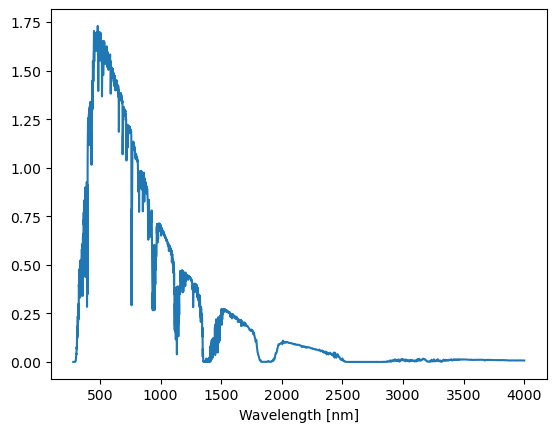
plt.plot(mi_espectra['Wvlgth'], mi_espectra['Direct_normal_irradiance'])
plt.xlabel('Wavelength [nm]')

Text(0.5, 0, 'Wavelength [nm]')

_images/d3b42e9f5cf10821b9ec8a1754b3cfb92cfd43dec57e526e85a583522b578990.png

Ahora plotea tanto la spectra directa como la difusa, poniendo el nombre de la columna de difusa abajo:

plt.plot(mi_espectra['Wvlgth'], mi_espectra['Direct_normal_irradiance'], label='Directa')
plt.plot(mi_espectra['Wvlgth'], mi_espectra[''], label='Difusa')   #<-- pon el nombre aqui
plt.xlabel('Wavelength [nm]')
plt.legend()

Ahora, vamos a integrar los espectras para saber el total de irradiación, usando una integración trapezoidal

from scipy import integrate

integrate.trapezoid(mi_espectra.Direct_normal_irradiance, x=mi_espectra.Wvlgth)

C:\Users\sayala\AppData\Local\Temp\1\ipykernel_13640\2096357368.py:3: DeprecationWarning: 'scipy.integrate.trapz' is deprecated in favour of 'scipy.integrate.trapezoid' and will be removed in SciPy 1.14.0
  integrate.trapz(mi_espectra.Direct_normal_irradiance, x=mi_espectra.Wvlgth)

1030.1432362323894

Vamos a imprimirlo de manera mas legible, y para ambos:

print("Irradiación Directa:", integrate.trapezoid(mi_espectra.Direct_normal_irradiance, x=mi_espectra.Wvlgth), "W/m\u00b2")
print("Irradiación Difusa:", np.round(integrate.trapezoid(mi_espectra.Difuse_horizn_irradiance, x=mi_espectra.Wvlgth),2), "W/m\u00b2")

Irradiación Directa: 1030.1432362323894 W/m²
Irradiación Difusa: 63.87 W/m²

Si te fijas, cuando imprimimos la irradiación Difusa, redondeamos el número a 2 dígitos, usando `np.round`.

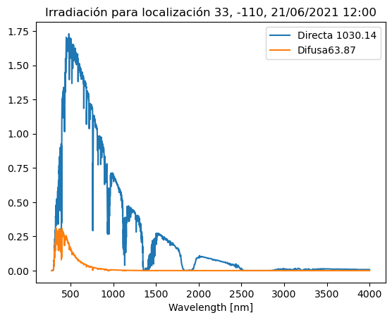
Por último, pongamos todo junto en una gráfica completa. 

#Grabemos como variables lo que calculamos arriba, para usarlo en los plots
int_directa = np.round(integrate.trapezoid(mi_espectra.Direct_normal_irradiance, x=mi_espectra.Wvlgth),2)
int_difusa = np.round(integrate.trapezoid(mi_espectra.Difuse_horizn_irradiance, x=mi_espectra.Wvlgth),2)
fecha = DAY+'/'+MONTH+'/'+YEAR+' '+HOUR+':00'     # Y tambien la fecha para poder usarla en el título

plt.plot(mi_espectra['Wvlgth'], mi_espectra['Direct_normal_irradiance'], label='Directa '+str(int_directa))
plt.plot(mi_espectra['Wvlgth'], mi_espectra['Difuse_horizn_irradiance'], label='Difusa'+str(int_difusa))   #<-- pon el nombre aqui
plt.xlabel('Wavelength [nm]')
plt.title('Irradiación para localización '+LATIT+', '+LONGIT+', '+fecha)
plt.legend()

<matplotlib.legend.Legend at 0x2a4b1f7ca70>

_images/6ed42734c631262d86b9e5c74edfab4586b51eb4ec88dcee25f28d9caf53de52.png

2. Plot Albedos from SMARTS#

IOUT = '30' # Albedo

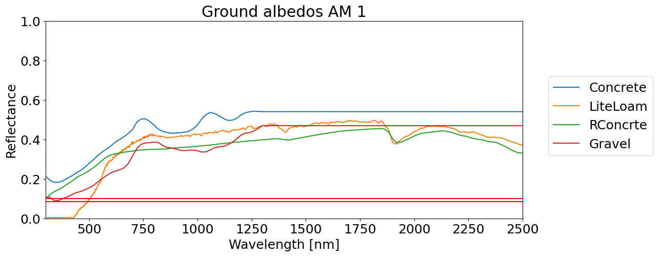
Plot Ground Albedo AM 1.0#

materials = ['Concrete', 'LiteLoam', 'RConcrte', 'Gravel']

alb_db = pd.DataFrame()

for i in range (0, len(materials)):

    alb = pySMARTS.SMARTSAirMass(IOUT=IOUT, AMASS='1.5', material=materials[i])

    alb_db[materials[i]] = alb[alb.keys()[1]]
    
alb_db.index = alb.Wvlgth

alb_db_10 = alb_db

for col in alb_db:
    alb_db[col].plot(legend=True)
    
plt.xlabel('Wavelength [nm]')
plt.xlim([300, 2500])
plt.axhline(y=0.084, color='r')
plt.axhline(y=0.10, color='r')

#UV albedo: 295 to 385
#Total albedo: 300 to 3000
#10.4 and 8.4 $ Measured
#References

plt.ylim([0,1])
plt.ylabel('Reflectance')
plt.legend(bbox_to_anchor=(1.04,0.75), loc="upper left")
plt.title('Ground albedos AM 1')
plt.show()

vis=alb_db.iloc[40:1801].mean()
uv=alb_db.iloc[30:210].mean()

print(vis)
print(uv)

_images/a970d81cd521296c16c67f400c2605932a4d4c9c93015f3e658b296cbda31359.png

Concrete    0.446679
LiteLoam    0.335459
RConcrte    0.329492
Gravel      0.348642
dtype: float64
Concrete    0.191439
LiteLoam    0.004157
RConcrte    0.132566
Gravel      0.098542
dtype: float64

Extra: Averaging Albedos for Visible and UV#

vis=alb_db.iloc[40:1801].mean()
uv=alb_db.iloc[30:210].mean()
print("Albedo on Visible Range:\n", vis)
print("Albedo on UV Range:\n", uv)

Albedo on Visible Range:
 Concrete    0.446679
LiteLoam    0.335459
RConcrte    0.329492
Gravel      0.348642
dtype: float64
Albedo on UV Range:
 Concrete    0.191439
LiteLoam    0.004157
RConcrte    0.132566
Gravel      0.098542
dtype: float64

Tip: If you want full spectrum averages, we recommend interpolating as the default granularity of SMARTS at higher wavelengths is not the same than at lower wavelengths, thus the 'step' is not the same.

r = pd.RangeIndex(2800,40000, 5)
r = r/10
alb2 = alb_db.reindex(r, method='ffill')
print("Albedo for all wavelengths:", alb2.mean())

Albedo for all wavelengths: Concrete    0.504434
LiteLoam    0.294001
RConcrte    0.267986
Gravel      0.420818
dtype: float64

# FYI: Wavelengths corresponding to the albedo before and after interpolating
"""
# Visible
alb_db.iloc[40] # 300
alb_db.iloc[1801] # 3000

# UV
alb_db.iloc[30] # 295
alb_db.iloc[210] # 385        

# Visible
alb2.iloc[40] # 300
alb2.iloc[5440] # 3000

# UV
alb2.iloc[30] # 295
alb2.iloc[210] # 385   
"""

'\n# Visible\nalb_db.iloc[40] # 300\nalb_db.iloc[1801] # 3000\n\n# UV\nalb_db.iloc[30] # 295\nalb_db.iloc[210] # 385        \n\n# Visible\nalb2.iloc[40] # 300\nalb2.iloc[5440] # 3000\n\n# UV\nalb2.iloc[30] # 295\nalb2.iloc[210] # 385   \n'

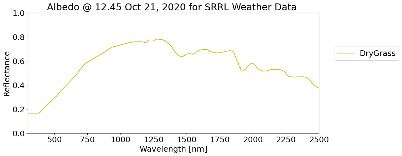
3. ADVANCED: Plot Ground Albedo for More Complete Weather Data#

This asumes you know a lot more parameters about your weather data souch as: Broadband Turbidity, Aeorsol Opticla Density parameters, and Precipitable Water.#

Real Input data from SRRL for OCTOBER 21st, 12:45 PM#

alb = 0.2205
YEAR='2020'; MONTH='10'; DAY='21'; HOUR = '12.75' 
LATIT='39.74'; LONGIT='-105.17'; ALTIT='1.0'; ZONE='-7'
TILT='33.0';  WAZIM='180.0'; HEIGHT='0' 
material='DryGrass'
min_wvl='280'; Max_wvl='4000'

TAIR = '20.3'
RH = '2.138'
SEASON = 'WINTER'
TDAY = '12.78'
SPR = '810.406'
RHOG = '0.2205'

WAZIMtracker = '270'
TILTtracker = '23.37'
tracker_tetha_bifrad = '-23.37'

TAU5='0.18422'     # SRRL-GRAL "Broadband Turbidity"
TAU5 = '0.037'    # SRRL-AOD [500nm]
GG = '0.7417'     # SSRL-AOD Asymmetry [500nm]
BETA = '0.0309'   # SRRL-AOD Beta
ALPHA = '0.1949'  # SRRL-AOD Alpha [Angstrom exp]
OMEGL = '0.9802'  # SRRL-AOD SSA [500nm]
W = str(7.9/10)   # SRRL-PWD  Precipitable Water [mm]

material = 'DryGrass'

alb_db = pd.DataFrame()

alb = pySMARTS.SMARTSSRRL(
    IOUT=IOUT, YEAR=YEAR, MONTH=MONTH,DAY=DAY, HOUR='12.45', LATIT=LATIT, 
    LONGIT=LONGIT, ALTIT=ALTIT, 
    ZONE=ZONE, W=W, RH=RH, TAIR=TAIR, 
    SEASON=SEASON, TDAY=TDAY, TAU5=None, SPR=SPR, 
    TILT=TILT, WAZIM=WAZIM,
    ALPHA1 = ALPHA, ALPHA2 = 0, OMEGL = OMEGL,
    GG = GG, BETA = BETA,
    RHOG=RHOG, HEIGHT=HEIGHT, material=material, POA = True)

alb_db[material] = alb[alb.keys()[1]]   
alb_db.index = alb.Wvlgth

alb_db[material].plot(legend=True, color='y')
plt.xlabel('Wavelength [nm]')
plt.xlim([300, 2500])
plt.ylim([0,1])
plt.ylabel('Reflectance')
plt.legend(bbox_to_anchor=(1.04,0.75), loc="upper left")
plt.title('Albedo @ 12.45 Oct 21, 2020 for SRRL Weather Data ')
plt.show()

_images/638cc329117d6495155af2a11295f227083e11967a0babcfffebecb68c3efa8c.png

A plotly plot to explore the results#

import plotly.express as px

fig = px.line(alb_db[material], title='Albedo @ 12.45 Oct 21, 2020 for SRRL Weather Data')

fig.update_layout(xaxis_title='Wavelength [nm]',
                  yaxis_title='Reflectance')
fig.show()