Welcome to Python, Jupyter, and Google Collab

How to use this tutorial?

This tutorial is a Jupyter notebook. Jupyter is a browser based interactive tool that combines text, images, equations, and code that can be shared with others. Please see the setup section in the README to learn more about how to get started.

Tutorial Structure

This tutorial is made up of multiple Jupyter Notebooks. These notebooks mix code, text, visualization, and exercises.

If you haven’t used JupyterLab before, it’s similar to the Jupyter Notebook. If you haven’t used the Notebook, the quick intro is

1. There are two modes: command and edit

2. From command mode, press Enter to edit a cell (like this markdown cell)

3. From edit mode, press Esc to change to command mode

4. Press shift+enter to execute a cell and move to the next cell.

5. The toolbar has commands for executing, converting, and creating cells.

The layout of the tutorial will be as follows:

# if running on google colab, uncomment the next line and execute this cell to install the dependencies and prevent "ModuleNotFoundError" in later cells:
# !pip install -r https://raw.githubusercontent.com/PVSC-Python-Tutorials/PVSC50/main/requirements.txt

Exercise: Print Hello, world!

Each notebook will have exercises for you to solve. You’ll be given a blank or partially completed cell, followed by a hidden cell with a solution. For example.

Print the text “Hello, world!”.

# Your code here
print("Hello, world!")

Hello, world!

Exercise 1: Modify to print something else:

my_string =    # Add your text here. Remember to put it inside of single quotes or double quotes ( " " or '' )
print(my_string)

  Cell In[3], line 1
    my_string =    # Add your text here. Remember to put it inside of single quotes or double quotes ( " " or '' )
                   ^
SyntaxError: invalid syntax

Let’s go over some Python Concepts

(A lot of this examples were shamely taken from https://jckantor.github.io/CBE30338/01.01-Getting-Started-with-Python-and-Jupyter-Notebooks.html :$)

Basic Arithmetic Operations

Basic arithmetic operations are built into the Python langauge. Here are some examples. In particular, note that exponentiation is done with the ** operator.

a = 2
b = 3
print(a + b)
print(a ** b)
print(a / b)

5
8
0.6666666666666666

Python Libraries

The Python language has only very basic operations. Most math functions are in various math libraries. The numpy library is convenient library. This next cell shows how to import numpy with the prefix np, then use it to call a common mathematical functions.

import numpy as np

# mathematical constants
print(np.pi)
print(np.e)

# trignometric functions
angle = np.pi/4
print(np.sin(angle))
print(np.cos(angle))
print(np.tan(angle))

3.141592653589793
2.718281828459045
0.7071067811865476
0.7071067811865476
0.9999999999999999

Lists are a versatile way of organizing your data in Python. Here are some examples, more can be found on this Khan Academy video.

xList = [1, 2, 3, 4]
xList

[1, 2, 3, 4]

Concatenation

Concatentation is the operation of joining one list to another.

x = [1, 2, 3, 4];
y = [5, 6, 7, 8];

x + y

[1, 2, 3, 4, 5, 6, 7, 8]

np.sum(x)

10

Loops

for x in xList:
    print("sin({0}) = {1:8.5f}".format(x,np.sin(x)))

sin(1) =  0.84147
sin(2) =  0.90930
sin(3) =  0.14112
sin(4) = -0.75680

Working with Dictionaries

Dictionaries are useful for storing and retrieving data as key-value pairs. For example, here is a short dictionary of molar masses. The keys are molecular formulas, and the values are the corresponding molar masses.

States_SolarInstallations2020 = {'Arizona': 16.04, 'California': 30.02, 'Texas':18.00, 'Colorado': 44.01}  # GW
States_SolarInstallations2020

{'Arizona': 16.04, 'California': 30.02, 'Texas': 18.0, 'Colorado': 44.01}

We can a value to an existing dictionary.

States_SolarInstallations2020['New Mexico'] = 22.4

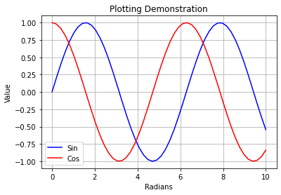
Plotting

Importing the matplotlib.pyplot library gives IPython notebooks plotting functionality very similar to Matlab’s. Here are some examples using functions from the

%matplotlib inline

import matplotlib.pyplot as plt
import numpy as np

x = np.linspace(0,10)
y = np.sin(x)
z = np.cos(x)

plt.plot(x,y,'b',x,z,'r')
plt.xlabel('Radians');
plt.ylabel('Value');
plt.title('Plotting Demonstration')
plt.legend(['Sin','Cos'])
plt.grid()

Now you’re ready

This skills will allow you to explore any jupyter notebook.

This work is licensed under a Creative Commons Attribution 4.0 International License.